> restart:

Graphing (One)

We shall try to examine various kinds of graphs. We start with an example in which we want to find out where the graph is rising and where it is falling.

Example 1.

> f:= x -> 8*x^4 - x^8;

> plot(f);

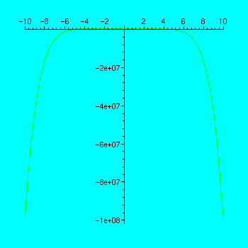
Note that Maple's default scaling doesn't give us much information about the behavior of the graph in some crucial regions. Finding the derivative to see where the function is increasing and decreasing may be helpful.

> f1:= D(f);

Since the derivative function is continuous, it can only change sign where it vanishes.

> solve(f1(x) = 0, x);

Zero is a multiple root. Two of the other roots are imaginary and can be ignored. The other three (including zero) are candidates for a sign change for the derivative. Let's examine the graph of the function more carefully near these points. In order to do so, we shall only look at the portion of the graph for between and 2, and we shall also limit the vertical range by specifying limits and for .

> c := -20;
d := 20;
plot(f(x), x=-2..2,y=c..d);

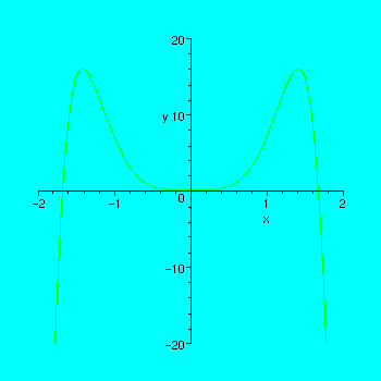
So the function increases up to , then decreases to zero, increases up to , and then decreases thereafter. This behavior was completely invisible in our first attempt to have Maple do the graphing for us. This is an example of where computer graphics used in partnership with the tools of calculus can elicit information that would otherwise not be easily available about the graph of a function.

>

Homework

Problem 1. Find an accurate graph of where . This graph also involves some very small ripples which might not be noticed if you didn't know where to look for them. You may do this simply by going back in the worksheet, changing the definition of the function and then making suitable changes in the following statements. Warning: you will have to fiddle quite a lot with the vertical limits and in order to be able to see the ripples. When you are done, give a verbal description below of the behavior of the function, including information about where it is increasing, where it is decreasing and where it attains local maxima and minima.

>

Asymptotes

One of the hardest things to get right is graphs with asymptotes which are either vertical lines which the graph approaches or are lines which the graph approaches as x approaches or . If the line is a vertical line, you may be able to detect it because the function has an infinite discontinuity for the relevant value of x.

Example 2 .

> f:= x-> (2*x^3 -3*x^2 +1)/(x^2 -9);

> plot(f);

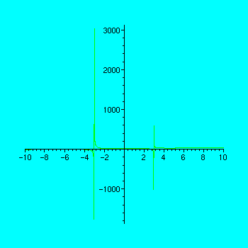
The "jags" in this graph are there because Maple is assuming that the function is continuous and trying to connect the graph over a vertical asymptote. We can get a better picture by scaling the axes.

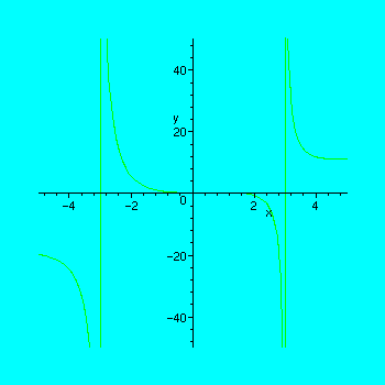
> plot(f(x), x=-5..5, y=-50..50);

>

But this is still not quite right because the vertical lines are not part of the graph. They are pretty close to the actual vertical asymptotes, so we get a slight dividend from Maple in this case . Note that these asymptotes occur when is undefined because its denominator is 0 (and its numerator is not 0). In this case, they occur when , i.e. when or , which is consistent with the plot above.

This graph has another kind of asymptote which we now want to investigate. To get a first look, let's plot the graph again for a very large range on the x-axis.

> plot(f(x), x=-100..100);

>

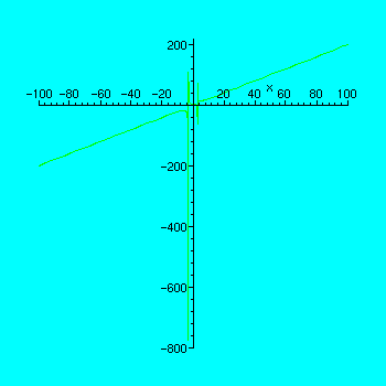
Notice at this scale the graph looks almost like a straight line except for some oscillation near the origin! You should now go back and change the scale to x=-1000..1000, which will have the effect of hiding what happens near the origin. Does the graph look exactly like a straight line now? That straight line is in fact an asymptote which the graph approaches as approaches . For large , the graph of the function is not identical with that line but is so close to it that Maple cannot distinguish the two.

>

Let's now find out what the equation of that line or asymptote is.

Define to be the slope of a line joining the point ( ) and the point (x, f(x)) .

> m:= (f(x) - f(0))/(x-0);

As x gets larger and larger this should get closer and closer to the slope of the desired line. So we calculate the limit of as goes to .

> limit(m, x=infinity);

So our line has an equation of the form and we would like to find the value of . We do that by calculating another limit of the difference between the function value and the value for a line of slope two through the origin.

> limit( 2*x - f(x), x=infinity);

This says for very large values of the value of is about 3 less than the value of . In other words is very close to for very large values of . Let's check that with another limit.

> limit( 2*x - 3 - f(x), x = infinity);

In other words the distance between the graph of the function and the graph of asymptotic line approaches as goes to .

Homework

Problem 2. In principle, the graph could approach some other line as approaches , and there are functions for which that can happen. Determine in this case if you get the same line as approaches . Do it by going back to the limit of and replace ` infinity ' by `-infinity' to see if you still get 2 as the limit. Similarly, determine if you also get the same value of by replacing `infinity' by `-infinity' in the calcuation of . Describe what you found below.